Introducing Parametric Probability Estimator

MartinLiebig

Feature preparation is one of the most challenging and important tasks in data science. The task has three facets

 

1. Preserve maximum information for best results
2. Reduce the number of attributes to a minimum for optimal runtime
3. Make the data easily understandable for the algorithm

With making the data easily understandable, you can get best performance. A given learner may be good in detecting some kind of patterns but might be blind for others. A good example are Generalized Linear Models (GLM), which are good in detecting linear patterns but not good in detecting non-linear pattern. The new Operator Univariate Probability Estimator is a useful addition to your toolkit for feature preparation.

 

Knowing your data

The first two tasks in the classical CRISP-DM cycle are business and data understanding. During these phases, an Analyst learns alot about a given task. With this information, he can often deduce reasonable assumptions on the attribute distributions. To put this into context, let us examine two examples.

In a customer analytics scenario, you may have an attribute NumberOfCalls. This covers the number of times you called the customer. From statistical knowledge, we can reasonably assume that this attribute is Poisson distributed.

In sensor analytics such as predictive maintenance, you often cope with a lot of measured data. Sensor responses are - thanks to the central limit theorem - often normally distributed.

 

Using this Information

In a classification task, we assume that the attributes have the power to distinguish between our classes. We can assume that both classes have one underlying distribution each. This distribution follows the same pattern (e.g. Normal distribution) but with different parameters. Now we can estimate the parameters of each class. In the binominal case, we get two distributions.

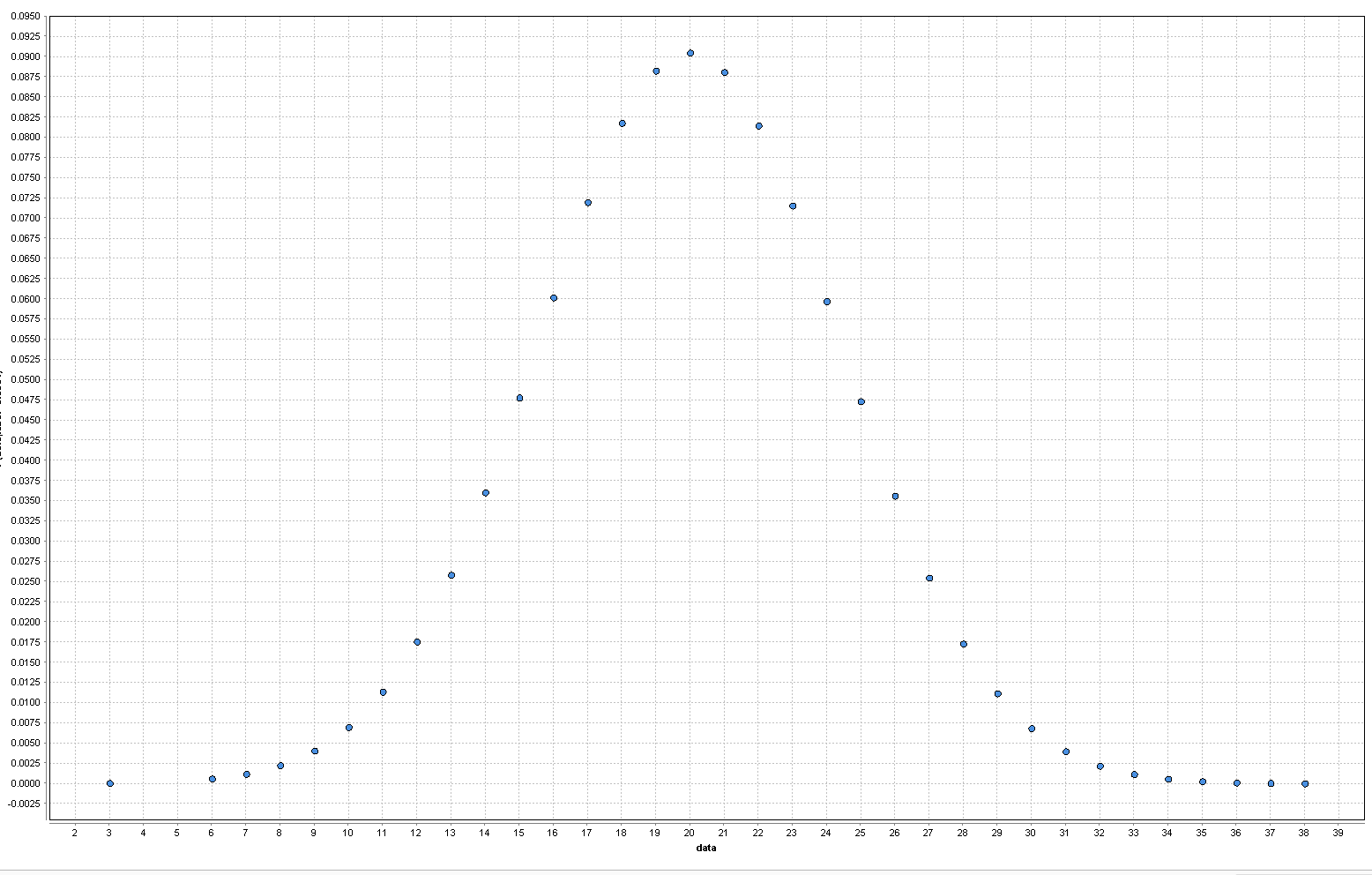
PDF of a Poisson Distribution. Low and High values are mapped to low probabilities while values around 20 have a high probabilityIf we take a value for a given example, we can calculate the probability that this value is fitting to one of these distributions. This results in two new attributes for our classification: 1) Probability that X belongs to FirstClassDistribution and 2) Probability that X belongs to SecondClassDistribution.

This is a non-linear feature transformation. For all distributions, consider two cases. On one hand, attribute values which are small or large compared to the mean are mapped to lower propabilities. On the other hand, values closer to the mean are mapped to higher probabilities. This results in a linearization of the problem. Linear models like GLM or Linear SVM can handle these values much easily than in their original form. The other effect is seen in tree based models such as Random Forests or GBTs, which can also handle this data better because they need less cuts for the same separation.

Using this in RapidMiner is straight forward with the new Operator called Univariate Probability Estimator. The settings are mainly the distribution assumption and the attributes to use it on. As of December 2017, we support the following distributions:

• Normal (aka Gaussian)
• Poisson
• LogNormal
• Exponential
• Bernoulli

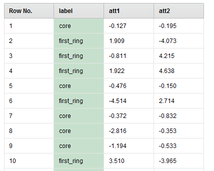
Consider this dataset:

Applying the Univariate Probability Estimator Operator on above dataset creates this output:

 

As sees, 2 new attributes are added for each previously existing attributes. These are the probability that a value in att1 or att2 belongs to a particular class.

The Operator also provides a preprocessing model. This model can be used to apply the same transformation on a different dataset. This is often necessary if you want to preprocess unknown data i.e. data similar to the original in structure but comprising of new examples unseen by the model.

The data shown above is a "ring dataset". Plotting att1 against att2 results in this chart:

We see that there is an outer ring around a normal distributed class. This dataset is not separable by a linear model.
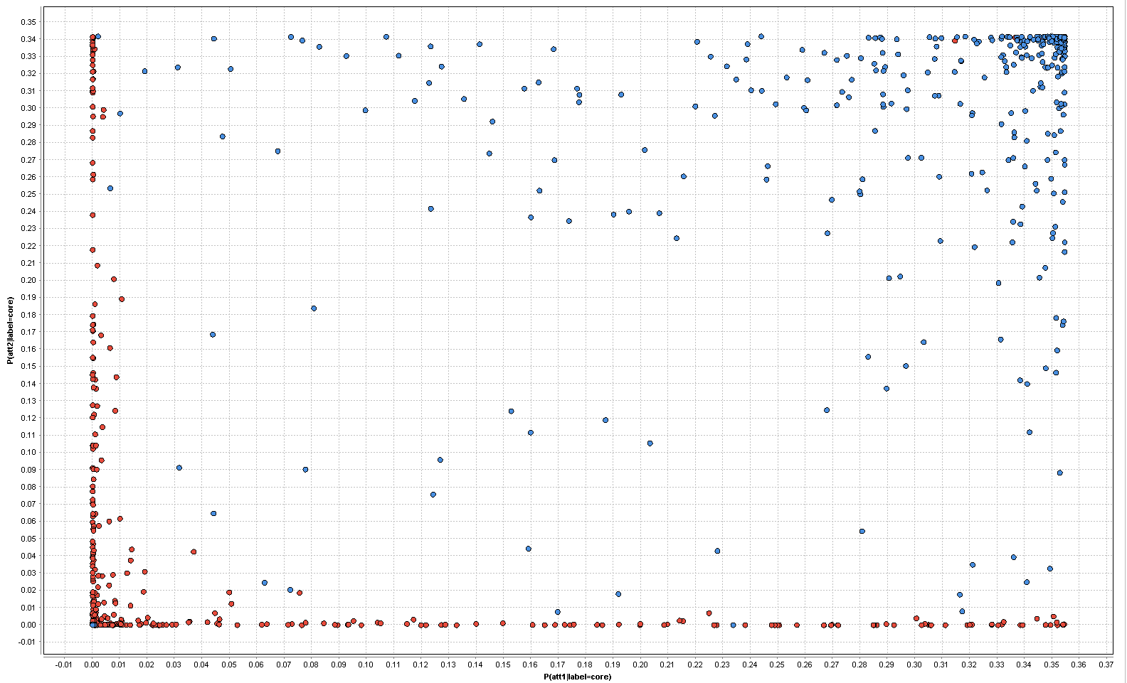
After the transformation we get four new attributes. If we just plot the P(att1|label=core) vs P(att2|label=core) on a plane, we get the following result:

In this plane, you can already see that a linear model can have a good success. Consequently, a Linear SVM with this transformation results in an AUC of 0.97 while the one without employing this transformation only achieves 0.43.

The described process is available as a tutorial process of the Univariate Probability Estimator Operator.