Credit Card Fraud Detection using Kaggle Data Set and Anomaly Detection
Anomaly Detection using Rapidminer and Python
I have always felt that anomaly detection could be a very interesting application of machine learning. I can think of several scenarios where such techniques could be used.
In this article I shall describe some experiments I carried out with the Credit Card Fraud Detection dataset from Kaggle. The dataset contains transactions made by credit cards in September 2013 by European cardholders over a two day period. There are 492 frauds out of a total 284,807 examples. Thus, the dataset is highly unbalanced, with the positive class (frauds) accounting for only 0.172% of all transactions. You can imagine that any such dataset would be highly unbalanced, as expected fraud or anomalous cases would only make up for a small percentage of the total transactions.
I carried out this analysis in two parts. First I under-sampled the dataset in Python by retaining all the fraud examples and by randomly selecting some amount of non-fraud examples such that in the final dataset the fraud cases had a good representation. In the second part, I used Rapidminer to develop models to predict the anomalous cases. Rapidminer is a GUI based platform for machine learning that makes it possible for you to design processes and workflows for building and evaluating models. You can even do so without a coding background and so I think it is a very useful tool for managers who want to apply these techniques quickly and realize value without having to struggle through excessive coding.
The original dataset itself can be downloaded from Kaggle at the link below [use this link].
As it is financial data, the features in the dataset are PCA transformations of the original features. So what you will see are only numerical values with no background information, the transactions are completely anonymous. The first column is the time in seconds, of each transaction from the first, I discarded this column in my analysis. Then there are 28 numerical features along with an Amount feature column which is the transaction amount. The final column is the Class in which the 1s are the fraud cases. This is the column that we would like our model to learn and be able to predict for new transactions.
 Dataset preview
Now the problem in such unbalanced datasets is that there are very few 1s in the Class column. These are the fraud cases that we want to be able to learn and predict. However if your model simply predicts 0s for all, you would still get a very high accuracy >99% because most transactions are not fraud anyway, but you will not be detecting any of the anomalies.
So instead of using the full dataset as is, I created a subset of the original dataset by well representing the fraud cases as an overall percentage of cases in the new dataset. This was done in Python as explained below.
# load required libraries
from numpy import concatenate
from pandas import read_csv
from pandas import DataFrame
from sklearn.preprocessing import MinMaxScaler
import pandas as pd
import numpy as np

num_features = 30 #Number of features in the dataset
label_feature = 'Class' #The column in dataset that model is being built to predict
The above libraries are required for this code
# Reading in the dataset which is in .csv format, has column headings and has an index column
dataset = read_csv("creditcard2.csv", header = 0, index_col = 0, squeeze = True, usecols = (i for i in range(0, num_features+1)))
Then the original .csv file of the Kaggle dataset is read, the first column have Time data is treated as an index column. This column only carries time information from the first transaction in the dataset and so I don’t think it is a useful feature that can be used for prediction.
scaler = MinMaxScaler(feature_range=(-1, 1))
dataset['normAmount'] = scaler.fit_transform(dataset['Amount'].reshape(-1, 1))
dataset = dataset.drop(['Amount'],axis=1)
Then I have used the MinMaxScaler to normalize the Amount column, which otherwise has a very different range of values as compared to the other columns. This is general good practice before using the data for machine learning. This new normalized column for Amount is retained and the original Amount column is dropped.
# Move label column to the end of dataset
cols_at_end = [label_feature]
dataset = dataset[[c for c in dataset if c not in cols_at_end] + [c for c in cols_at_end if c in dataset]]
I generally use the above code to move the label column to the end of the dataset, it makes it easy to read and to separate it out if required. In this case it is already at the end so the above code makes no change.
# Number of datapoints belonging to the minority class
number_fraud = len(dataset[dataset.Class == 1])

fraud_indices = np.array(dataset[dataset.Class == 1].index)

# Finding out the indices of the normal class
normal_indices = dataset[dataset.Class == 0].index


# Out of the normal indices, randomly select fraud number of occurences
random_normal_indices = np.random.choice(normal_indices, number_fraud, replace = False)

random_normal_indices = np.array(random_normal_indices)

# Appending the 2 sets of indices
under_sample_indices = np.concatenate([fraud_indices, random_normal_indices])

# Under sample dataset from the selected indices
under_sample_data = dataset.loc[under_sample_indices,:]
The above code gets the number of fraud cases in the original dataset and then selects randomly an equal number of non-fraud examples to build a 50:50 under sampled dataset. If you look closely the above code has an error. It is to do with the .loc operand, it does not exactly perform what we are intending and I was unable to resolve this. But I was still getting an under sampled dataset with close to 28% representation of fraud cases and so I went ahead. Maybe at some future point I can resolve this error.
under_sample_data.to_csv('Undersampled.csv', encoding='utf-8', index=False)
Finally we export the under sampled dataset into a .csv file which will be used in Rapidminer for the remainder of the analysis. So from here on we are working in Rapidminer Studio.
 RapidMiner process flow
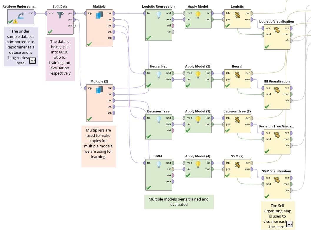
The process implemented in RapidMiner is shown above (you can also open it directly in RapidMiner here). With the RapidMiner interface it is pretty easy to see and understand what is happening. The operators used above are drag and drop, making it very easy to implement. We make a 80:20 split of the under sampled dataset with shuffling, and use multiple copies of this to train multiple predictors. Each of the learnt model is applied on the 20% validation split and the results obtained. I have also used the Self Organising Map (SOM) for visualisation operator to actually visualize the learnt models.
I have compared 4 techniques: Logistic regression, which is the default choice for such binomial classification tasks, a Neural Network, Decision Tree and Support Vector Machine. The process runs in under one minute and the results are given below:


From the above results it can be seen that each of the models are doing a really good job with their predictions. The accuracy is pretty good. The logistic regression is the best performer. So its really that simple to build an anomaly detection system! Some cases of frauds are being missed out and some further fine tuning may be required.
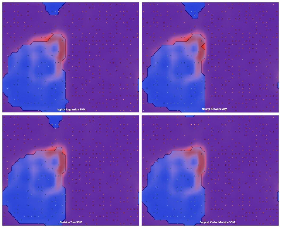
The Self Organizing Maps for visualization operators help visualize the learnt models by reducing them to a two dimensional space. The summary of the four visualizations are shown below, with each dot representing the predicted class. The boundaries can be clearly observed, showing the learnt classification. You can also observe the dots that are bright orange in color or light blue, these are the few cases of erroneous predictions.
 SOM visualizations
With this there is one final step to be completed and that is to use the entire dataset and apply the learnt models and see how it performs for the full data. The process is similar to the Rapidminer process shown above except that instead of the 20% split data copies you use the original dataset. The studio version can only work on 10,000 datapoints but that should be good enough. The results obtained are below.


It can be seen that while the Logistic regression and Neural network model capture all fraud cases they also predict false positives, which may lead to large number of investigation of non-fraud cases. While the Decision Tree and SVM models make far fewer false positive predictions they do also miss out one actual fraud case. One will have to make a call on which model to use based on these results. Perhaps investigations can be carried out depending on the transaction amount, or maybe use an ensemble of models for prediction.
This technique can be applied to other areas — anomalous applications for insurance, anomalous checklist filling etc. The true difficulty lies in capturing the right data that can make good features as part of the dataset used for training, and this is where planning and creativity is required.
Hope this article has been an interesting read!

 Contributor II
Answers
@sgenzer
Hi, I was trying to study and understand the process you have here, but get stuck in connections. I am a novice to RM.
1- why do you have 2 Multiply? could not find where the second one connected to.
2- can we use cross validation to compare different models instead of having them here?
Thanks
Laleh
hello @laleh_moradi - the Split Data operator splits the data set into two pieces. One Multiply is used for one partition, the other for the other partition. And no, x-validation is used to properly build one model, not to compare models.
There are LOTS of training materials on these topics - have you checked out our "Training" section and our "Getting Started" section? These are good places to learn these techniques.
Scott
or logistic visualization, NN visualization and decitiontree Visulisation and svm visulisation...
2-multiply connection (2) It is not known where to attach it ??? can you send for me a clearer picture of the implementation
Scott
Fariba
I have a problem with the labels? Is there anyone who can help with it? Thanks